This work is conducted in collaboration with Prof. Sharon H. Ackerman and Prof. Elisabeth R. Tillier. We maintain a Matlab Toolbox (MSAVOLVE) for the simulation and detection of coevolution from multiple sequence alignments (MSAs).
MSAVOLVE v3.0a can be donwloaded HERE.
During the past decade many efforts have been devoted to uncover the evolutionary dynamic of organisms through the examination of multiple sequence alignments (MSA’s). The MSA of the members of a protein family provides a 2-dimensional view of a protein history, in which the 3rd and 4th dimensions, structure and time, are flattened. In a MSA some positions are highly conserved, while others vary. For example, the destabilizing effects of a given amino acid at one position can be compensated by the stabilizing effect of a certain amino acid at another position. The existence of physical and functional interactions between sites in protein sequences leads to non-independence of their evolution: in other words, two (or more) positions in a protein sequence could be coevolving, and for any mutation to become fixed at such sites, compensatory mutations are needed at the related sites.
However, a high background of different interacting factors often hides the coevolutionary relationships between amino acid sites. A simple model to explain the correlation Cij between two sites i and j in a sequence alignment was proposed by Atchley et al.:
Cij = Cphylogeny + Cstructure + Cfunction + Cinteraction + Cstochastic
In this model Cphylogeny is the correlation originating from phylogenetic relationships between homologous sequences that belong to the same branch of an evolutionary tree. For example, a mutation in an ancestral protein, which is clearly a single evolutionary event, appears in the MSA as an independent event that occurred in each of the proteins that descended from that ancestor. Cstructure and Cfunction represent the correlation originating from structural and functional constraints. Ultimately, the preservation of structure is also related to the preservation of function because small changes in atom distances in the active site (produced by overall changes of structure) can have effects on the binding and activation energies as dramatic as those produced by very localized mutations in the active sites. As a consequence, these sources of correlation, which are the most important signal that coevolution analyses try to extract from the MSA, are typically not independent from one another. Furthermore, as mutations are fixed elsewhere in the sequence throughout the evolutionary process, the functional and structural constraints on the correlation between sites may even change. Cinteraction describes both the interaction between the aforementioned sources of correlation, and the correlation originating from atomic interactions in homo-oligomeric proteins. Finally, Cstochastic represents the correlation originating from casual co-variation and/or from uneven or incomplete sequence sampling. Low-quality and poorly populated MSAs are likely to produce a high degree of false coevolution signals as a result of the significant effect of stochasticity.
A wide variety of algorithms have been developed to detect coevolving positions from a MSA. In practice, most approaches to correlated mutation analysis do not discriminate between structural and functional correlations, and the sensitivity of most of parametric and non-parametric methods to detect these two forms of coevolution (the important signal) is ultimately dependent on the quality of the MSA, and is compromised in various degrees by the ability of these methods to filter out the stochastic and phylogenetic noise.
Another problem shared by most methods that use co-evolution analysis to predict interactions among residues is that many structurally distant pairs appear to be strongly correlated. One source of this correlation is the phylogenetic relationship between sequences in a multiple alignment. Another source is the propagation of statistical dependencies along chains of co-evolving contacts, which tends to confound direct with indirect interactions. Disentanglement of these two types of interactions was achieved with the application of Bayesian network modeling to the MIP algorith, and most recently with the application of Direct Coupling Analysis (DCA, a maximum entropy method based on the hypothesis that the probability of observing a certain sequence in an MSA depends on the Boltzmann distribution of this sequence in terms of its total energy, and that this energy depends on the interaction between coevolving pairs), and with the application of a sparse inverse matrix in the calculation of partial correlation with PSICOV.
In the absence of an analytical model for covariation, many studies have relied on the simulations of MSAs as a tool to test a method capacity to filter out the background coevolution signal. Simulated MSAs can reproduce some of the evolutionary parameters of the real MSA (e.g., the level of conservation and the amino acid distribution at each site, the distribution of pair-wise similarities between individual sequences) and thus, given a certain amino acid substitution model, can easily yield the true coevolution signal. In our own attempts to develop a simulation protocol with these characteristics, we have noticed that the outcome of the simulations is dependent on the assumptions that are made by the program with regard to how the protein is evolved, how coevolution is defined and counted, and how coevolving residues are chosen. Also, earlier simulations of MSAs developed for the purpose of studying coevolution have not included recombination processes (e.g., horizontal transfers), which by their own nature can produce large coevolving blocks inside a protein. In nature, protein families have developed as a result of the continuous process of random mutations, recombination and selection, which tends to eliminate most destabilizing mutations. Recombination plays a key role in the natural evolution of proteins because it explores a part of sequence space that is particularly rich in folded and functional proteins, leading to the swapping of well-defined structural domains. The accumulated experience of directed evolution studies indicates that also during laboratory evolution, as in nature, recombination promotes the rapid accumulation of beneficial mutations from multiple parents onto a single offspring. For this reason, we have developed a new program, MSAvolve (implemented as a Matlab Toolbox and distributed under BSD licensing), for the in silico evolution of MSAs, which allows for both substitutions at individual sites, and recombination in and between branches of an evolutionary tree. The evolved MSAs attempt to replicate the evolutionary parameters derived from the MSAs of real protein families. The choice of strictly covarying positions and of recombination segments is defined in detail and highly customizable.
In all cases MSAvolve records a history of all covarying positions, and automatically builds a total coevolution matrix (hereon named ‘totCOV’) as the accumulated sum of individual matrices for the positions that were forced to co-vary (covarion coevolution, ‘covCOV’ matrix), the positions that coevolved as a consequence of recombination (recombinant coevolution, ‘recCOV’ matrix), and those that coevolved by pure chance (stochastic or random coevolution, ‘mutCOV’ matrix).
In this context, it is worth noting some important features of MSAvolve, like the capacity of simulating MSAs with uneven branch sizes, and that of analyzing mutation, coevolution, and recombination events in only some parts – a branch or a specific group of sequences – of the evolutionary tree. In particular, the automatic branch assignment of MSAvolve can satisfy a user’s request to identify clusters in the experimental MSA using more than 2 principal components (PCs) of the covariance or other type of distance matrix.
Altogether, MSAvolve generates a large number of MSAs that mimic the statistical properties of the experimental one (regardless of whether the ancestor is created using the background frequencies of amino acids in the family or the HMM emission probabilities), although each MSA is distinctly different from every other one. This feature of the program can be conveniently exploited to test the capacity of different algorithms to detect correctly pairs of residues that are truly coevolving regardless of the large variety of other background covariations that can occur because of phylogenetic or stochastic associations. In particular, MSAvolve builds coevolution matrices of each simulated MSA by counting the mutations that segregate at specific times during the evolution of a protein. This function can be equated to that of an external observer that witnesses the historical process of evolution. With respect to this point there are two observers in MSAvolve: one is a ‘low power’ observer, who counts all the co-segregating mutations regardless of whether they originate from chance, recombination, or functional/structural demands (the latter are the mutations under constraint of coevolution). There is also a ‘high power’ observer, who counts selectively the true co-segregating mutations of functional/structural significance.
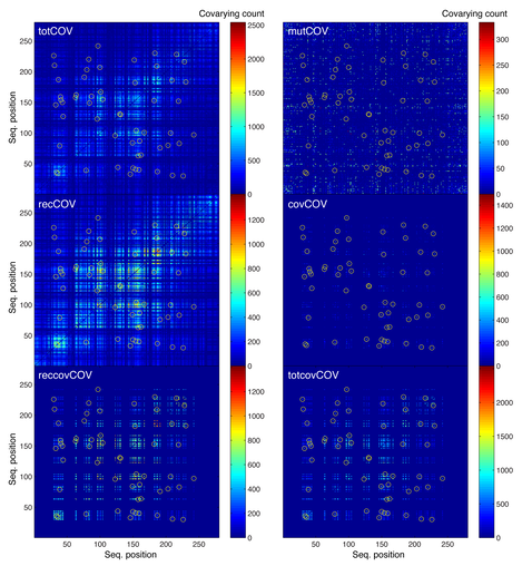
An example of the information gathered by the observers (as reported in the construction of coevolution matrices) is shown for a typical MSA generated by MSAvolve. The panel labeled ‘totCOV’ represents the total count of all the coevolution events. The residue pairs that are under constraint of coevolution are indicated by yellow circles. A detailed description of how the count is carried out is described in the Methods section. The panel labeled ‘mutCOV’ represents the count of the coevolution events due to random point mutations at positions that are not set to coevolve. MSAvolve prevents random mutations from occurring at positions that belong to a covarion pair: when a residue belonging to a covarion pair happens to be selected for mutation, then the other residue in the pair is also automatically selected for mutation. In this way the ‘random’ mutations and the ‘covarions’ mutations are always kept separate. The panel labeled ‘recCOV’ represents the count of coevolution events due to recombination; since recombination affects simultaneously large blocks of sequence, its effects on the coevolution count are much larger that those of point mutations.
The matrix labeled ‘covCOV’ is the count of the true covarions. In this matrix there are counts also at pairs of positions that were not set to be covarying. This is due to the fact that when by chance two or more covarion pairs mutate and segregate during an arbitrary amount of time, also the cross-count between pairs are added. For example if pairs 12-34 and 70-93 both mutate, then the count increases by 1 not only for those two pairs but also for the pairs 12-70, 12-93, 34-70, and 34-93. Since are not always the same pairs that mutate at the same time, the background from cross-pairs counts is not as high as the count from the true covarying pairs. On the other hand, the cross-pairs count is also amplified by the recombination process. This can be seen in the panel labeled ‘reccovCOV’, which shows the count of all the coevolution events produced by recombination at both the true covarion pairs and at the cross-covarion pairs. The coevolution signal is significantly degraded in this matrix. Summing the ‘covCOV’ and ‘reccovCOV’ matrices produces a matrix of the total coevolution signal from which all effects of stochastic coevolution have been removed: this matrix is shown in the panel labeled ‘totcovCOV’. Returning to our analogy, the ‘low power’ observer sees only the ‘totCOV’ matrix, whose coevolution signal is quite contaminated. Only the ‘high power’ observer sees the ‘covCOV’ matrix, but there are limits even to its powers because the coevolution signal is not completely clean even in this matrix.
We notice here that, while the individual matrices are built independently during the simulated evolution of the MSA from a single ancestor, in the end they are all consistent with each other: for example, a matrix identical to the totCOV matrix is obtained independently as the sum of the mutCOV, covCOV, and recCOV matrices.
Detection of covariation in simulated alignments
The calculated coevolution matrices shown above describe in full the true coevolutionary history of the MSA generated by MSAvolve, and can be compared with those derived for the same MSA by some of the leading methods to detect coevolution. A measure of how well different methods (including MSAvolve own totCOV and covCOV matrices) identify covarying pairs in the entire set of 100 simulated MSAs is shown below as the distribution among these MSAs of the percentage of true covarions in the top 28 zscores (the actual number of true covarions) of each matrix. This is a traditional measure of sensitivity. The dashed grey and orange lines reflect the counts of actual covariation events made that the hidden observers inside MSAvolve. For example, among the MI methods , ZPX2 does just as well as the ‘low power’ observer (which sees only the totCOV matrix). In this case, DCA and the binary ZPX2 methods all exceed the performance of ZPX2, with nbZPX2 doing almost as well as the ‘high power’ observer (which sees the covCOV matrix). But even this observer does not recognize correctly every true covariation event: as we mentioned, this is due to contamination of the coevolution signal in this matrix by stochastic cross-covariation between true covarions. In general, non-MI methods, like the very popular Statistical Coupling Analysis (SCA), do very poorly, as their performance is worse than simple MI.
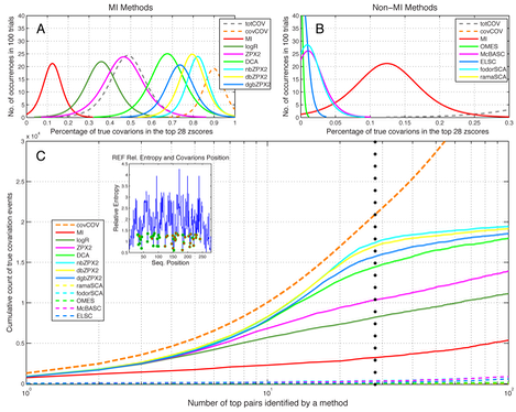
A. Distributions among 100 MSAs of the percentage of true covarions in the top 28 zscores of each matrix of different MI methods. Only the fits to the actual distributions are shown. The dashed grey and orange lines represent respectively the counts of covariation events made by the hidden observers inside MSAvolve. The ‘low power’ observer (grey line) sees only the totCOV matrix; the ‘high power’ observer sees the covCOV matrix. B. Same as panel A, but for non-MI methods. C. Cumulative count of covariation events corresponding to the top scoring pairs in the coevolution matrices generated by different methods. A dotted vertical line marks the 28th highest scoring pair. The inset shows the relative entropy of the experimental MSA with superimposed the covarions position.
Another measure of sensitivity can be obtained by using the actual counts of the true coevolution events for each pair provided by the covCOV matrices as the values for the corresponding pairs identified by the different methods. In this analysis the ij pairs of the covCOV matrix and the ‘method’ matrix are first sorted in descending order based on their value. Then, the values of the ij pairs of the covCOV matrix are assigned to the corresponding ij pairs of the ‘method’ matrix. For example, if pair 20:40 was counted 500 times in the covCOV matrix the corresponding pair 20:40 of the ‘method’ matrix is assigned a value of 500 regardless of its original value. In this way a plot of the cumulative sum of the values of the sorted ‘method’ matrix visualizes how much the coevolution recognition provided by the method approaches the ‘ideal’ coevolution recognition provided by the cumulative sum of the values of the sorted covCOV matrix. The result of this analysis averaged over all 100 simulated MSAs in the set is shown in the lower panel of the figure.
Analysis of X-ray crystal structures
The generation of simulated MSAs of protein families for which a representative X-ray structure is available allows us to address the issue of whether residue pairs that are expected to be coevolving based on their closeness in 3-dimensional space represent the totality or just a subset of all coevolving positions, and whether different coevolution detection methods are preferentially detecting one or the other. To quantify the detection of coevolving residues that are close in space, we can measure what percentage of all residue pairs separated by less than 8 Å in the X-ray structure is represented in the top coevolving pairs identified by each method. This result can be further filtered in order to include only pairs whose component residues are separated by at least 1, 5, 10 or more positions in sequence space. The result of this analysis for the experimental MSA and X-ray structure of 8 different proteins (KDO8PS, ARSC, ARSA, ATP11P, ATP12P, PDR, PHBH, MDH) is shown below.
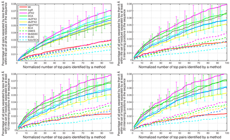
Each panel shows the percentage in the top coevolving pairs identified by each method, among the residue pairs separated by less than 8 Å in the X-ray structure of each protein. The abscissa scale is normalized in such a way that 100 corresponds to a number of pairs equal to the number of residues in the sequence. In the top left panel all protein pairs are considered, including those represented by consecutive residues in the sequence. In the top right panel only pairs whose residues are separated by at least 5 intervening positions in sequence space are considered. In the bottom left and bottom right panels only pairs whose residues are separated by at least 10 and 20 intervening positions in sequence space are considered.
Flowchart of the simulation of MSAs with MSAvolve.
MSAvolve v.2.0a is implemented as a Matlab Toolbox under BSD licensing. In order to run smoothly it requires the Bioinformatics, Statistics, and Curve Fitting Toolboxes for Matlab. Given a real MSA of a protein family, MSAvolve generates one or more artificial MSAs that mimic the statistical properties (e.g., sequence profile, pairwise similarity distribution, conservation at each position) of the real MSA.
Although it is possible to build ancestor sequences of arbitrary length, in most cases, the MSA simulation starts with reading the experimental MSA of a real protein family and converting it to a numeric format (each aa is represented by a number between 1 and 20, gaps are represented as number 21). The total length (including gaps) of each aligned sequence in the real MSA defines the length of each sequence in the simulated MSA. First, a Hidden Markov Model (HMM) of the real MSA is built: the HMM provides the emission probabilities and background frequencies of the 20 amino acids at each position in the MSA. A non-parametric kernel smoothing distribution with a smoothing bandwidth of 0.01 is fitted to the vector of emission probabilities for each position of the MSA. An object representing the fitted distribution is stored for each MSA position, and an ancestor sequence is built by random drawing (rounded to the nearest integer) from the probability distribution of each position. Alternatively, MSAvolve can be prompted to produce an ancestor also from the equilibrium frequencies.
Next, a phylogenetic tree built from the matrix of pairwise distances is used to determine the number of main branches in the real MSA, which will be replicated in the simulated MSA (an arbitrary number of branches can however be set manually). Several options are available to calculate pairwise distances and trees, as offered in the Matlab Bioinformatics Toolbox (which is required for MSAvolve to function). Alternatively, branches can be determined from a spectral analysis of the covariance matrix of the sequences in the MSA.
Once the number and size of the main branches are decided, identical copies of the ancestral sequence become the starting point for populating the nodes of the evolutionary tree. Next a certain percentage of the position in the sequence is selected as covarying pairs. These pairs represent the positions that in a natural evolution would be under structural and/or functional constraints. Therefore, correlated evolution of these positions is the source of the most important signal that we seek to extract in coevolution analyses. Pairs can be selected in a strictly random fashion or based on the entropy (or relative entropy) of positions in the real MSA. For example, if we want 10% of all positions in a sequence of 300 aa’s to be covarying with another 10%, we can select two vectors of 30 indices (the covarying matrix) corresponding to the columns in the MSA with the largest (or smallest or intermediate levels of) entropy. A non-parametric kernel smoothing distribution with a smoothing bandwidth of 0.01 is fitted to the vector of the joint probabilities of any two aa’s at the covarying positions in the real MSA. An object representing the fitted distribution is stored for each covarying pair (a row in the covarying matrix). If the evolution tree is split into branches (reflecting the branches of the experimental MSA), different objects representing the fitted distribution of the same selected covarying pairs are built for each branch.
MSAvolve adopts a fixed 3-LEVELS architecture with each level containing alternating steps (epochs or periods) of point mutations and steps of recombination to generate the final MSA. Each level represents an expansion of the evolutionary tree. While the program could have been designed with an arbitrary number of levels, in early testing we found that additional levels were only slowing down the execution time without changing the final outcome. Thus, while the general architecture is fixed (only 3 levels), inside each level all the steps can be repeated an arbitrary number of times with arbitrary parameters, giving rise to a very high degree of flexibility in balancing the amount of point mutations against the amount of recombination in and between branches. As an example we describe here the generation of a MSA corresponding to an evolutionary tree with 3 main branches and 45 sequences each of 300 residues.
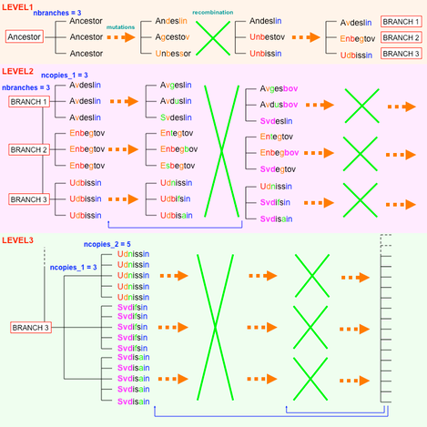
LEVEL 1: the simulation starts with 3 identical copies of the ancestor (only the first 8 residues of the ancestor are shown). Each copy is subjected to n cycles of point mutations. Each cycle represents an arbitrary amount of time at the end of which a certain amount of changes in the sequence of the ancestor has become fixed. In each cycle and for each copy of the ancestor the mutational rate is chosen randomly from within a chosen range of values (e.g. 2-5%). The range of target rates used in the default setting of MSAvolve do not reflect known mutational rates of one or more particular organisms, but have been optimized by trial and errors in order to produce simulated MSAs that in most cases mimic well the experimental MSAs. However, the user can adjust the range of the target rates at will.
In practice, the protein is evolved inside a single matrix containing 3 identical rows corresponding to the ancestral protein. For example, if for a certain row we want to achieve a target mutational rate of 5% we will generate a random number from a Poisson distribution assuming that 5% of all the sequence positions may have changed during the mutation cycle. Thus the target number of mutations (l of the Poisson distribution) is 300 x 0.05 = 15. We draw a number from this distribution once for each sequence in the MSA. Then, for each sequence we draw the positions that must change from a uniform distribution of 300 positions: these positions are stored in a “random mutation vector”. If any of these positions corresponds to a column in the MSA that is listed in the “global (or branch) covarying matrix”, that position is pulled out of the random mutation vector and added to the first column of a “cycle covarying matrix”. The second column of this matrix is completed retrieving the other element of each pair from the global covarying matrix.
At the beginning of the evolution process, the 3 sequences in the matrix are identical to the ancestral sequence , but they will start diverging as mutations accumulate. For each of the three sequences in the MSA, the positions defined by the random mutation vector are evolved first by random drawing from the aa probability distribution of each of these positions in the real MSA, as determined previously (see above). The covarying pairs are evolved next by random drawing from the joint aa probability distribution of these pairs in the real MSA, as determined previously (see above). It can be seen here how by always drawing each aa change from the observed probability distribution of aa’s at each position or from the observed joint probability distribution at each pair of positions, the profile of the evolved MSA becomes progressively more similar to the profile of the real MSA, although individual sequences may be significantly different. Once the changes in all the sequences are completed (corresponding to the fixing of all mutations during the arbitrary amount of time represented by a mutation cycle) they are simply counted and added to a coevolution matrix; for example if there was a change at position 20 and a change at position 121, the value of the coevolution matrix at the position with indices [20,121] is increased by 1. A separate coevolution matrix is maintained for the random mutations and for the mutations in coevolving pairs. With regard to the latter it should be mentioned that if in a mutation cycle more than one covarying pair becomes fixed, the coevolution matrix will reflect additional cross-changes between pairs: for example if pairs [10,15] and [34,70] both change, the coevolution matrix will record an increase by 1 at indices [10,15], [34,70], [10,34], [10,70], [15,34], [15,70]. We have decided to keep the coevolution matrices for the random mutations and for the true coevolving pairs separate, but one could argue that the correct count of the true correlation between positions at the end of each mutational cycles should include also the cross-correlation between random mutations and covarying mutations. Doing so dramatically increases Cstochastic with respect to Cstructure/function, and represents one of the possible user choices that affect the interpretation of the simulation. At any rate, MSAvolve also calculates a “global coevolution matrix” (this is the ‘glob_COV’ variable in the simulation output) that incorporates the cross-correlation between random mutations and co-varying positions.
An important parameter for the simulation is the ratio between mutational rate in each cycle and number of consecutive cycles. The same overall number of mutational changes can be obtained with different combinations of these numbers as long as their product remains approximately constant. However, since the counting of co-evolution takes place at the end of each mutational cycle (which we equate to the segregation of all mutations after a certain amount of time), having fewer cycles with more mutations increases Cstochastic with respect to Cstructure/function. On the other end, cycles cannot be made arbitrarily small, because it would imply that no mutations are ever deleterious (any mutation is fixed), and in the limit, from the practical standpoint of how the programs works, all mutations would appear to be the product of functional or structural coevolution. This effect can be exploited by the user to test the ‘strength’ of a coevolution detection method. Weaker methods are expected to detect progressively fewer true covarions than stronger methods as the mutational rates increases, and the number of cycles decreases. Furthermore, since the mean entropy of the columns in the MSA grows monotonically with the overall mutation rate, to simulate data that are analogous to a given real MSA, it is useful to find a value of the product “mutation_rate x mutation_cycles” that gives an entropy similar to that of the real data. However, as previously discussed, while the final MSAs obtained maintaining this product constant will have the same column entropy, the corresponding coevolution matrices will have significantly different levels of Cstochastic.
MSAvolve alternates rounds of mutations (consisting of multiple mutation cycles) with rounds of recombination. In the beginning of our example recombination occurs between the three branches of the MSA (Figure 13; at this point each branch is represented by just one sequence). The recombination process implemented in MSAvolve is the unidirectional transfer of a contiguous block of aa’s from one sequence to one or more other sequences. It is meant to simulate the spread of a successful block of residues among the members of the family. It is critical to define how the recombination blocks are chosen. We have explored two strategies: in one strategy the sequence is split in a finite number of blocks whose boundaries are selected by randomly drawing from a uniform distribution of the indices of all positions. This strategy is very convenient if a simulated MSA is generated multiple times (e.g. 100 times) for the purpose of collecting coevolution statistics, in which case having different recombination fragments in different simulations spreads the effects of recombination evenly throughout a sequence. A second strategy requires knowledge of the three-dimensional structure of at least one member of the real MSA. In this second case the SCHEMA algorithm can be used to predict which fragments of homologous proteins can be recombined without disturbing the integrity of the structure.
Once the cross-over point are defined, MSAvolve carries out recombination in two steps:
1. It selects at random the number and identity of the sequences that will receive the donated fragment.
2. It selects at random which fragment will be donated and which sequence will donate the fragment to the other sequences.
Usually, within one round of recombination, multiple cycles of recombination are carried out, each with a different random selection of the donor, the recipients, and the donated fragment. Each recombination cycle represents an arbitrary amount of time after which the effects of the recombination process are fixed in the MSA. At the end of each recombination cycle the changes in all the sequences are simply counted and added to a recombination coevolution matrix; for example a fragment encompassing positions [5,6,7,8,9,10] may have spread from sequence 3 to sequence 1 and 2. If this spread produces a change at positions [5,6] in sequence 1 and positions [5,6,9] in sequence 2, the recombinant coevolution matrix will report an increase by 2 at indices [5,6] and an increase by 1 at indices [5,9] and [6,9].
The 1st level of the MSA simulation is completed by another round of point mutations such that altogether the flowchart of this level is: point mutations -> recombination -> point mutations (flowchart, orange section).
LEVEL 2: this level starts expanding the tree to bring it to the final expected size of 45 sequences. For example, to achieve the desired number of sequences we can multiply the original 3 sequences by 3 at level 2 and by 5 at level 3. In practice, at level 2 two copies of each of the 3 sequences of level 1 are added to the MSA matrix, which now contains 9 rows and 3 different sequences (the original 3 branches of the tree) derived from a single ancestral protein. The corresponding coevolution matrices are expanded accordingly by multiplication of the original counts.
The flowchart of level 2 is: mutations in each sequence -> recombination between all the sequences regardless of the branch they belong to -> mutations in each sequence -> recombination between sequences of each branch -> mutations in each sequence (flowchart, pink section ).
LEVEL 3: 4 copies of each of the 9 sequences of level 2 are added to the MSA matrix, which now contains 45 rows and 9 different sequences (3 for each of the original 3 branches of the tree) derived from a single ancestral protein. The corresponding coevolution matrices are expanded accordingly by multiplication of the original counts.
The flowchart of level 3 is: mutations in each sequence -> recombination between all the sequences inside each of the 3 main branches -> mutations in each sequence -> recombination between sequences inside each of the 9 sub-branches -> mutations in each sequence (flowchart, green section).
The 3-level architecture of the program reflects the hypothesis that as the protein family expands and the members diverge recombination between members of distant branches of the tree becomes more difficult. Once all levels of MSAvolve are completed, the global and/or individual coevolution matrices can be analyzed and compared to those derived from the final fully evolved MSA by an external program. It is also possible to select randomly or (not randomly) only certain sequences of the evolved MSA, in which case the corresponding coevolution matrices are also made available. This feature allows the effect of Cphylogenetic to be readily evaluated.
Coevolution detection methods.
A very large number of coevolution detection methods is currently implemented in MSAvolve v3.0a. They are:
MI, MIP, ZRES, ZPX, ZPX2, nb/db/dgb, 3D_MI, 4D_MI, DCA, plmDCA, gplmDCA, hp_pca_DCA, PSICOV, slPSICOV, GREMLIN, logR, OMES, McBASC, ELSC, SCA.
Key papers:
The contribution of coevolving residues to the stability of KDO8P synthase
SH Ackerman, DL Gatti
PloS one 6 (3), e17459
SH Ackerman, ER Tillier, DL Gatti
PloS one 7 (10), e47108
Clark GW, Ackerman SH, Tillier ER, Gatti DL.
BMC Bioinformatics. 2014 May 22;15:157.
Gatti DL
Current Topics In Biochemical Research, 16, 67-79, 2015
Tools for the Simulation and Detection of Coevolving Positions in Multiple Sequence Alignments
Gatti DL
Current Biotechnology, 4(1): 16-25, 2015